Acquiring the CCE module
There are a couple different ways to acquire the CCE module/executable.
From a release
Starting from late May 2024, in every Release of SpECTRE we offer a tarball that contains everything needed to run CCE on a large number of different systems. This will be under the Assets section towards the bottom of the release (there may be a lot of text detailing what's been updated in this release). Inside this tarball is
- the CCE executable CharacteristicExtract
- an example YAML input file
- an example set of Bondi-Sachs worldtube data in the Tests/ directory (see Input worldtube data formats section)
- example output from CCE in the Tests/ directory
- a PreprocessCceWorldtube executable and YAML files for converting between worldtube data formats in the PreprocessCceWorldtube/ directory
- a WriteCceWorldtubeCoordsToFile executable that writes grid points on a sphere to a text file in the PreprocessCceWorldtube/ directory
- a python script CheckCceOutput.py (meant to be run from the root of the tarball and after you run the example YAML input file also in the root of the tarball) that will check if the example output is correct
- Note
- The tarball is .xz so use tar -xf TarName.tar.xz to extract. The -z flag to use gzip will cause an error.
See Running the CCE executable for how to run CCE.
We have tested that this executable works natively on the following machines:
- Expanse
- Anvil
- Stampede3
- Delta (if you add LD_LIBRARY_PATH=/sw/spack/deltas11-2023-03/apps/linux-rhel8-x86_64/gcc-8.5.0/gcc-11.4.0-yycklku/lib64/:$LD_LIBRARY_PATH before running CCE)
- Perlmutter
- Ubuntu 18.04 LTS or later (LTS version only)
We have also tested that this executable works inside our dev Docker container on the following machines (in addition to the ones above):
- Frontera
- Delta
From Docker
You can download a docker image sxscollaboration/spectre:deploy which has a few pre-built executables within, including the ones listed above in the release section. See the containerized releases section of our Installation instructions for how start the container.
The input files can be found within the container at /work/spectre/tests/InputFiles/.
From source
You can clone the spectre repo and follow the instructions on the Installation page to obtain an environment to configure and build SpECTRE. Once you have a configured build directory, build the CCE executable with
- Note
- You may want to add the -j4 flag to speed up compilation. However, be warned that this executable will need several GB of memory to build.
Input worldtube data format
In order to run the CCE executable, the worldtube data must be represented as Bondi-Sachs variables decomposed as a subset of spin-weighted spherical harmonic modes on a sphere of constant coordinate radius. We have chosen this format because it is far more space-efficient to store on disk than other formats. This section will detail the required data format, provide options for converting worldtube data from other NR codes into our format, and give insights into what the worldtube data should look like.
Required H5 worldtube data format
Within the H5 file that holds the worldtube data, there must be the following datasets with these exact names (including the .dat suffix):
- Beta.dat
- DrJ.dat
- DuR.dat
- H.dat
- J.dat
- Q.dat
- R.dat
- U.dat
- W.dat
Each dataset in the file must also have an attribute named Legend which is an ASCII-encoded null-terminated variable-length string. That is, the HDF5 type is:
This can be checked for a dataset by running
For the ordering of the data, we use spherical harmonic conventions documented by the ylm::Spherepack class. Each row must start with the time stamp, and the remaining values are the complex modes in m-varies-fastest format. For spin-weight zero Bondi variables (Beta, R, DuR, W), we omit the redundant negative-m modes and imaginary parts of the m=0 modes to save space on disk. Here is an example of a legend for the spin-weight zero variables:
For non-zero spin-weight Bondi variables (J, DrJ, H, Q, U) we must store all complex m-modes. Here is an example of a legend for variables where all complex m-modes must be specified:
We don't have strict requirement on the name of the H5 file that holds the worldtube data. However, it is recommended to name the H5 file ...CceRXXXX.h5, where the XXXX is to be replaced by the zero-padded integer for which the extraction radius is equal to XXXXM. For instance, a 100M extraction should have filename ...CceR0100.h5. If you do not adhere to this naming convention, you will need to specify the extraction radius in your YAML input file.
- Note
- This scheme of labeling files with the extraction radius is constructed for compatibility with worldtube data from the SXS Collaboration's SpEC code.
Converting to the required H5 format
Unless you are using worldtube data that was generated from SpECTRE (or SpEC), it's possible that your worldtube data is not in the correct format. We allow conversion into our data format from a few other data formats using the `PreprocessCceWorldtube` executable provided. These are
- Nodal cartesian metric data (which we refer to as "metric nodal")
- Modal cartesian metric data (which we refer to as "metric modal")
- Nodal Bondi-Sachs data (which we refer to as "bondi nodal")
Requirements for these data formats are listed below.
Spherical harmonic modes
When we refer to a "modal" data format, we mean that the worldtube data are stored as spherical harmonic coefficients (a.k.a. modes). We use spherical harmonic conventions documented by the ylm::Spherepack class. For each dataset, each row must start with the time stamp, and the remaining values are the complex modes in m-varies-fastest format. That is,
Each dataset in the H5 file must also have an attribute named Legend which is an ASCII-encoded null-terminated variable-length string.
Spherical harmonic nodes
When we refer to a "nodal" data format, we mean that the worldtube data are stored as values at specially chosen collocation points (a.k.a. grid points or nodes). This allows SpECTRE to perform integrals, derivatives, and interpolation exactly on the input data. These grid points are Gauss-Legendre in \(cos(\theta)\) and equally spaced in \(\phi\).
Below is a routine for computing the spherical harmonic \(\theta\) and \(\phi\) values. These can be used to compute the Cartesian locations for a given radius using the standard transformation. The routine supports \(\ell\in[4, 32]\).
C Code for computing SpECTRE CCE gridpoint locations
Alternatively, if your code can read in grid points from a text file, you can run the WriteCceWorldtubeCoordsToFile executable like so to get a text file with three columns for the x,y,z coordinates of each point.
Each dataset holds 1 + (l_max + 1) * (2 * l_max + 1) columns, with the first one being the time. The columns must be in \(\theta\)-varies-fastest ordering. That is,
Each dataset in the H5 file must also have an attribute named Legend which is an ASCII-encoded null-terminated variable-length string.
- Note
- Nodal data is likely the easiest to write out since no conversion to spherical harmonic coefficients is necessary.
ADM Cartesian metric and derivatives
For worldtube data stored in an H5 file in the "ADM metric nodal" format, there must be the following datasets with these exact names (including the .dat suffix):
- gxx.dat, gxy.dat, gxz.dat, gyy.dat, gyz.dat, gzz.dat
- Dxgxx.dat, Dxgxy.dat, Dxgxz.dat, Dxgyy.dat, Dxgyz.dat, Dxgzz.dat
- Dygxx.dat, Dygxy.dat, Dygxz.dat, Dygyy.dat, Dygyz.dat, Dygzz.dat
- Dzgxx.dat, Dzgxy.dat, Dzgxz.dat, Dzgyy.dat, Dzgyz.dat, Dzgzz.dat
- Shiftx.dat, Shifty.dat, Shiftz.dat
- DxShiftx.dat, DxShifty.dat, DxShiftz.dat
- DyShiftx.dat, DyShifty.dat, DyShiftz.dat
- DzShiftx.dat, DzShifty.dat, DzShiftz.dat
- Lapse.dat, DxLapse.dat, DyLapse.dat, DzLapse.dat
- Kxx.dat, Kxy.dat, Kxz.dat, Kyy.dat, Kyz.dat, Kzz.dat
- Either: AuxiliaryShiftx.dat, AuxiliaryShifty.dat, AuxiliaryShiftz.dat
- Or: ConformalChristoffelx.dat, ConformalChristoffely.dat, ConformalChristoffelz.dat
Here g represents the spacetime metric, but we only require the spatial components (e.g. gxx.dat, gxy.dat, etc...) so in practice, those are the tensor components of the spatial metric. The temporal components of the spacetime metric are stored separately in the lapse and shift. Each of the spatial metric, lapse, and shift must also have their cartesian derivatives. K is the extrinsic curvature, AuxiliaryShift is the auxiliary shift vector used in the first-order form of the Gamma-driver condition, and ConformalChristoffel is the trace of the conformal second_order symbols.
We will compute the time derivative of the spatial metric using Eq. (2.134) of [14],
\begin{equation}\partial_t \gamma_{ij} = -2\alpha K_{ij} + D_i\beta_j + D_j\beta_i. \end{equation}
The time derivative of the lapse is computed using the 1+log slicing condition from Eq. (4.87) of [14]
\begin{equation}\partial_t \alpha = -2\alpha K + \beta^j\partial_j\alpha, \end{equation}
and the time derivative of the shift is computed using either the first order reduction form of the Gamma-driver condition from Eq. (4.89) of [14]
\begin{equation}\partial_t \beta^i = \eta B^i + \beta^j\partial_j\beta^i, \end{equation}
where you can choose \(\eta\) (typically \(\eta=0.75\)) or using the integrated Gamma-driver condition from Eq. (12) of [103]
\begin{equation}\partial_t \beta^i = \tilde{\Gamma}^i - \eta\beta^i + \beta^j\partial_j\beta^i, \end{equation}
again, where you can choose \(\eta\) (typically \(\eta=2/M_{\textrm{ADM}}\)).
- Warning
- If your worldtube data is in the ADM metric nodal format but you have not used 1+log slicing and the Gamma-driver conditions specified above, your time derivatives will be wrong. If you'd like us to support other commonly used gauge conditions (or variants of 1+log or Gamma-driver), please open an issue on our GitHub.
The layout of each of these datasets must be spherical harmonic nodes.
Cartesian metric and derivatives
For worldtube data stored in an H5 file in either the "metric nodal" or "metric modal" formats, there must be the following datasets with these exact names (including the .dat suffix):
- gxx.dat, gxy.dat, gxz.dat, gyy.dat, gyz.dat, gzz.dat
- Drgxx.dat, Drgxy.dat, Drgxz.dat, Drgyy.dat, Drgyz.dat, Drgzz.dat
- Dtgxx.dat, Dtgxy.dat, Dtgxz.dat, Dtgyy.dat, Dtgyz.dat, Dtgzz.dat
- Shiftx.dat, Shifty.dat, Shiftz.dat
- DrShiftx.dat, DrShifty.dat, DrShiftz.dat
- DtShiftx.dat, DtShifty.dat, DtShiftz.dat
- Lapse.dat
- DrLapse.dat
- DtLapse.dat
Here g represents the spacetime metric, but we only require the spatial components (e.g. gxx.dat, gxy.dat, etc...) so in practice, those are the tensor components of the spatial metric. The temporal components of the spacetime metric are stored separately in the lapse and shift. The layout of each of these datasets must be in either spherical harmonic modes or spherical harmonic nodes.
Bondi-Sachs
In the "bondi nodal" format, you must have the same Bondi variables as the required format, but each variable layout must be the spherical harmonic nodal layout with complex values interleaved as Re, Im, Re, Im, ...
If you already have data in the required "bondi modal" format, then nothing needs to be done.
Running the PreprocessCceWorldtube executable
The PreprocessCceWorldtube executable should be run on any of the allowed input formats, and will produce a corresponding Bondi-Sachs worldtube file that can be read in by CCE. This executable works similarly to our other executables by accepting a YAML input file:
with a YAML file
In addition to converting worldtube data formats, PreprocessCceWorldtube also accepts multiple input worldtube H5 files that have sequential times (e.g. from different checkpoints) and will combine the times from all H5 files alongside converting the worldtube data format. If there are duplicate or overlapping times, the last/latest of the times are chosen. If you pass multiple input worldtube H5 files, it is assumed that they are ordered increasing in time.
Here are some notes about the different options in the YAML input file:
- If the extraction radius is in the InputH5File names, then the ExtractionRadius option can be Auto. Otherwise, it must be specified.
- The option LMaxFactor determines the factor by which the resolution of the boundary computation that is run will exceed the resolution of the input and output files. Empirically, we have found that LMaxFactor of 3 is sufficient to achieve roundoff precision in all boundary data we have attempted, and an LMaxFactor of 2 is usually sufficient to vastly exceed the precision of the simulation that provided the boundary dataset.
- FixSpecNormalization should always be False unless you are using a particualy old version of SpEC
- DescendingM should always be False. This option is to support metric modal data from SpEC. Our data format is always in ascending m.
- BufferDepth is an advanced option that lets you load more data into RAM at once so there are fewer filesystem accesses.
- If using the ADM metric nodal input data format with a first-order form gamma driver, specify the InputDataFormat: like so: InputDataFormat:AdmMetricNodal:Lapse:Advective: TrueShift:Advective: TrueFirstOrderDriverFactor: 0.75 # Eq. 4.89 B&S
- If using the ADM metric nodal input data format with an integrated gamma driver, specify the InputDataFormat: like so: InputDataFormat:AdmMetricNodal:Lapse:Advective: TrueShift:Advective: TrueConformalChristoffelFactor: 1.0 # Eq. 12 Hilditch 2013SecondOrderDriverEta: 2.0 # Eq. 12 Hilditch 2013
What Worldtube data "should" look like
While no two simulations will look exactly the same, there are some general trends in the worldtube data to look for. Here is a plot of some modes of the Bondi variable J from the Bondi-Sachs worldtube format.
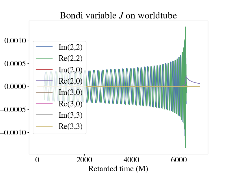
The 2,2 modes are oscillatory and capture the orbits of the two objects. The real part of the 2,0 mode contains the gravitational memory of the system. Then for this system, all the other modes are subdominant.
If you are using the cartesian metric or adm cartesian metric worldtube format, here is a plot of the imaginary part of the 2,2 mode of the lapse and its radial and time derivative during inspiral.
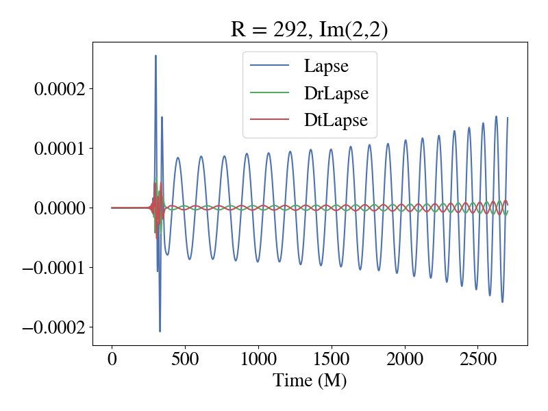
One thing to keep in mind with this plot is that it was produced using the Generalized Harmonic formulation of Einstein's equations using the damped harmonic gauge. Therefore, if you are using a different formulation and gauge (like BSSN + moving punctures), the lapse may look different than this. One way to sanity check your data (regardless of what type it is or where you got it from) is to look and how the mode amplitude for a given quantity decays as you increase (l,m). Here is a plot of the amplitude of the modes for the lapse in the above plot.
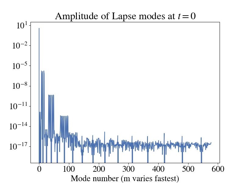
You'll notice that most modes are around machine precision and only the first few have any real impact. This is expected.
Input file for CCE
Input files for CCE are commonly named CharacteristicExtract.yaml. An example input file with comments explaining some of the options can be found in $SPECTRE_HOME/tests/InputFiles/Cce/CharacteristicExtract.yaml. Here we expand a bit on why we chose some of those parameters.
General options
- For resolution, the example input file has lmax (Cce.LMax) of 20, and filter lmax (Filtering.FilterLMax) of 18; that may run a bit slow for basic tests, but this value yields the best precision-to-run-time ratio for a typical BBH system. Note that precision doesn't improve above lmax 24, filter 22 (be sure to update the filter as you update lmax – the filter should generally be around 2 lower than the maximum l to reduce possible aliasing).
- If you want to just run over all times in the worldtube H5 file, you can set both the StartTime and EndTime to Auto and it will automatically figure it out based on the data in the worldtube file.
- The ScriOutputDensity adds extra interpolation points to the output, which is useful for finite-difference derivatives on the output data, but otherwise it'll just unnecessarily inflate the output files, so if you don't need the extra points, best just set it to 1.
- For production level runs, it's recommended to have the Cce.Evolution.StepChoosers.Constant option set to 0.1 for an accurate time evolution. However, if you're just testing, this can be increased to 0.5 to speed things up.
- We generally do not recommend extracting at less than 100M due to the CCE junk radiation being much worse at these smaller worldtube radii. That being said, we also recommend running CCE over several worldtube radii and checking which is the best based on the Bianchi identity violations. There isn't necessarily a "best radius" to extract waveforms at.
- Most users will not need it, but if you want to dump data from the volume (instead of only on future null infinity), this is possible with the ObserveFields option to Events within EventsAndTriggersAtSlabs in the input file. See the input file referenced above for a (commented-out) example, and the documentation of the class Cce::Events::ObserveFields for details.
Initial data on the null hypersurface
Choosing initial data on the initial null hypersurface is a non-trivial task and is an active area of research. We want initial data that will reduce the amount of CCE junk radiation as much as possible, while also having the initial data work for as many cases as possible.
SpECTRE currently has four different methods to choose the initial data on the null hypersurface. In order from most recommended to least recommended, these are:
- ConformalFactor: Try to make initial time coordinate as inertial as possible at \(\mathscr{I}^+\) with a smart choice of the conformal factor. This will work for many cases, but not all. But will produce the best initial data when it does work.
- InverseCubic: Ansatz where \(J = A/r + B/r^3\). This is very robust and almost never fails, but contains a lot of CCE junk radiation compared to ConformalFactor.
- ZeroNonSmooth: Make J vanish. Like the name says, it's not smooth.
- NoIncomingRadiation: Make \(\Psi_0 = 0\); this does not actually lead to no incoming radiation, since \(\Psi_0\) and \(\Psi_4\) both include incoming and outgoing radiation.
Rechunking worldtube data
- Note
- This section is less important than the others and really only matters if you will be doing a large number of CCE runs like for a catalog. For only a couple runs or just for testing, this part is unnecessary and can be skipped.
CCE will run faster if the input worldtube hdf5 file is chunked in small numbers of complete rows. This is relevant because by default, SpEC and SpECTRE write their worldtube files chunked along full time-series columns, which is efficient for writing and compression, but not for reading in to CCE. In that case, you can rechunk the input file before running CCE for maximum performance. This can be done, for instance, using h5py (you will need to fill in filenames appropriate to your case in place of "BondiCceR0050.h5" and "RechunkBondiCceR0050.h5"):
The rechunked data will still be in the same format as before, but will just have a different underlying structure in the H5 file that makes it faster to read in.
Running the CCE executable
Once you have acquired an executable, running CCE in a supported environment is a simple command:
You may notice at the beginning you get some warnings that look like
This is normal and expected. All it means is that initially an angular solve didn't hit a tolerance. We've found that it never really reaches the tolerance of 1e-13, but we still keep this tolerance so it gets as low as possible.
After this, you'll likely see some output like
which tells you that the simulation is proceeding as expected. When the run finished, you'll see something like
In terms of runtime, we've found that for a ~5000M long cauchy simulation, CCE takes about 6 hours to run. This will vary based on a number of factors like how long the cauchy evolution actually is, the desired error tolerance of your characteristic timestepper, and also how much data you output at future null infinity. Therefore, take these numbers with a grain of salt and only use them as a rough estimate for how long a job will take.
- Note
- CCE can technically run on two (2) cores by adding the option ++ppn 2 to the above command, however, we have found in practice that this makes little-to-no difference in the runtime of the executable.
Output from CCE
Once you have the reduction data output file from a successful CCE run, you can confirm the integrity of the h5 file and its contents by running
For the reduction file produced by a successful run, the output of the h5ls should resemble
Notice that the worldtube radius will be encoded into the subfile name.
- Note
- Prior to this Pull Request, merged May 15, 2024, the output of h5ls looked like this / Group/Cce Group/Cce/EthInertialRetardedTime.dat Dataset {3995/Inf, 163}/Cce/News.dat Dataset {3995/Inf, 163}/Cce/Psi0.dat Dataset {3995/Inf, 163}/Cce/Psi1.dat Dataset {3995/Inf, 163}/Cce/Psi2.dat Dataset {3995/Inf, 163}/Cce/Psi3.dat Dataset {3995/Inf, 163}/Cce/Psi4.dat Dataset {3995/Inf, 163}/Cce/Strain.dat Dataset {3995/Inf, 163}/src.tar.gz Dataset {3750199}
No matter the spin weight of the quantity, the \(\ell = 0,1\) modes will always be output by CCE. Also, the /SpectreR0100.cce group will have a legend attribute that specifies the columns.
Raw CCE output
The Strain represents the asymptotic transverse-traceless contribution to the metric scaled by the Bondi radius (to give the asymptotically leading part), the News represents the first time derivative of the strain, and each of the Psi... datasets represent the Weyl scalars, each scaled by the appropriate factor of the Bondi-Sachs radius to retrieve the asymptotically leading contribution.
The EthInertialRetardedTime is a diagnostic dataset that represents the angular derivative of the inertial retarded time, which determines the coordinate transformation that is performed at future null infinity.
If you'd like to visualize the output of a CCE run, we offer a CLI that will produce a plot of all of quantities except EthInertialRetardedTime. To see how to use this CLI, run
If you'd like to do something more complicated than just make a quick plot, you'll have to load in the output data yourself using h5py or our spectre.IO.H5 bindings.
- Note
- The CLI can also plot the "old" version of CCE output, described above. Pass --cce-group Cce to the CLI. This option is only for backwards compatibility with the old CCE output and is not supported for the current version of output. This options is deprecated and will be removed in the future.
Frame fixing
You may notice some odd features in some of the output quantities if you try and plot them. This is not a bug in CCE (not that we know of at least). This occurs because the data at future null infinity is in the wrong Bondi-Metzner-Sachs (BMS) frame. In order to put this data into the correct BMS frame, the SXS Collaboration offers a python/numba code called scri to do these transformations. See their documentation for how to install/run/plot a waveform at future null infinity in the correct BMS frame.
Below is a plot of the imaginary part of the 2,2 component for the strain when plotted using the raw output from SpECTRE CCE and BMS frame-fixing with scri. You'll notice that there is a non-zero offset, and this component of the strain doesn't decay back down to zero during the ringdown. This is because of the improper BMS frame that the SpECTRE CCE waveform is in. A supertranslation must be applied to transform the waveform into the correct BMS frame. See [149] for a review of BMS transformations and gravitational memory. To perform the frame fixing, see this tutorial in scri.
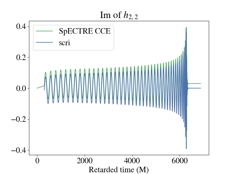
The discrepancy is even more apparent if you plot the amplitude of the two waveforms. It's pretty clear which waveform is the more "physical" one.
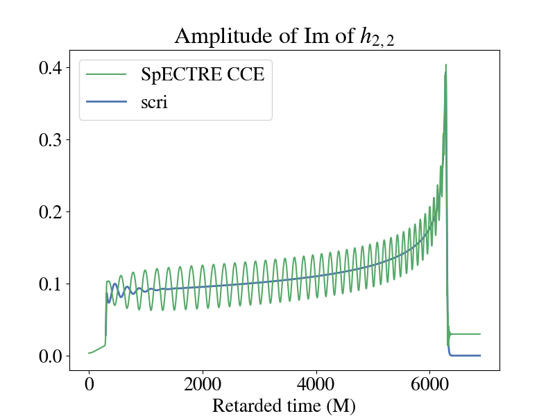
Notice that there are still some oscillations in the strain output by scri towards the beginning of the waveform (up to ~1500M). This is caused by CCE junk radiation from imperfect initial data on the null hypersurface. In order to use this waveform in analysis, the CCE junk must be cut off from the beginning.
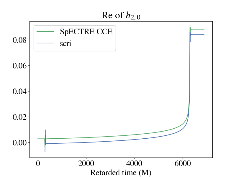
You are also able to see gravitational memory effects with SpECTRE CCE! This shows up in the real part of the 2,0 mode of the strain. Though you can see the memory effects in the SpECTRE CCE waveform, in order to do any analysis, you must also transform the waveform to a more physically motivated BMS frame.
Citing CCE
If you use the SpECTRE CCE module to extract your waveforms at future null infinity, please cite the following:
- SpECTRE DOI (This link defaults to the latest release of SpECTRE. From there, you can find links to past releases of SpECTRE as well)
- SpECTRE CCE paper
- CCE paper
If you used scri to perform any frame-fixing, please also consult the scri GitHub for how you should cite it.
You can also consult our Publication policies page for further questions or contact spectre-devel@black-holes.org.