Introduction

Each element in a domain has a set of internal directions which it uses for computations in its own local coordinate system. These are referred to as the logical directions \(\xi\), \(\eta\), and \(\zeta\), where \(\xi\) is the first dimension, \(\eta\) is the second dimension, and \(\zeta\) is the third dimension. In a domain with multiple Blocks, the logical directions are not necessarily aligned on the interfaces between two Blocks, as shown in the figure below. As certain operations (e.g. fluxes, limiting) communicate information across the boundaries of adjacent elements, there needs to be a class that takes into account the relative orientations of elements which neighbor each other. This class is OrientationMap.

%OrientationMaps between %Blocks

Each Block in a Domain has a set of BlockNeighbors, which each hold an OrientationMap. In this scenario, the Block is referred to as the host, and the OrientationMap held by each BlockNeighbor is referred to as "the orientation the BlockNeighbor has with respect to the host Block." This is a convention, so we give an example of constructing and assigning the correct OrientationMaps:

Two neighboring blocks.

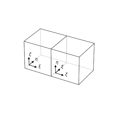
In the image above, we see a domain decomposition into two Blocks, which have their logical axes rotated relative to one another. With the left block as the host Block, we see that it has a neighbor in the \(+\xi\) direction. The host Block holds a std::unordered_map from Directions to BlockNeighbors; the BlockNeighbor itself holds an OrientationMap that determines the mapping from each logical direction in the host Block to that in the neighboring Block. That is, the OrientationMap takes as input local information (i.e. logical directions in the host's coordinate system) and returns neighbor information (i.e. logical directions in the neighbor's coordinate system). An OrientationMap is constructed by passing in the block neighbor directions that correspond to the \(+\xi\), \(+\eta\), \(+\zeta\) directions in the host. In this case, these directions in the host map to the \(+\zeta\), \(+\xi\), \(+\eta\) directions in the neighbor, respectively. This BlockNeighbor thus holds the OrientationMap constructed with the list ( \(+\zeta\), \(+\xi\), \(+\eta\)). With the right block as the host block, we see that it has a BlockNeighbor in the \(-\zeta\) direction, and the OrientationMap held by this BlockNeighbor is the one constructed with the array ( \(+\eta\), \(+\zeta\), \(+\xi\)). For convenience, OrientationMap has a method inverse_map which returns the OrientationMap that takes as input neighbor information and returns local information.

OrientationMaps need to be provided for each BlockNeighbor in each direction for each Block. This quickly becomes too large of a number to determine by hand as the number of Blocks and the number of dimensions increases. A remedy to this problem is the corner numbering scheme.

Encoding BlockNeighbor information using Corner Orderings and Numberings

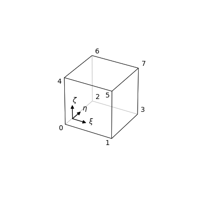
The orientation of the \({dim}\) logical directions within each element determines an ordering of the \(2^{dim}\) vertices of that element. This is called the local corner numbering scheme (Local CNS) with respect to that element. We give the ordering of the local corners below for the case of a three-dimensional element:

The local corner numbering.

Corner 0 is the location of the lower xi, lower eta, lower zeta corner.
Corner 1 is the location of the upper xi, lower eta, lower zeta corner.
Corner 2 is the location of the lower xi, upper eta, lower zeta corner.
Corner 3 is the location of the upper xi, upper eta, lower zeta corner.
Corner 4 is the location of the lower xi, lower eta, upper zeta corner.
Corner 5 is the location of the upper xi, lower eta, upper zeta corner.
Corner 6 is the location of the lower xi, upper eta, upper zeta corner.
Corner 7 is the location of the upper xi, upper eta, upper zeta corner.

What remains is to endow the domain decomposition with a global corner numbering (Global CNS). We give an example below:

A global corner numbering.

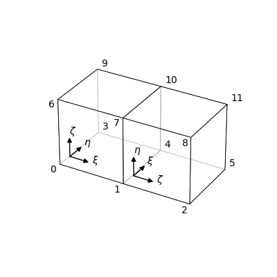
In the image above, we see that each vertex of the two-block domain has been assigned a number. Although each block has eight corners, four are shared among them, so there are only twelve unique corners in this domain. Any numbering may be used in the global corner numbering, so long as the each distinct corner is given a single distinct corner number.

Note: This Global CNS assumes that there is no additional identifying of faces with one another for periodic boundary conditions. That is, each element must have \(2^{dim}\) distinct corner numbers. If you wish to additionally identify faces of the same block with each other, that must be done in an additional step. This step is explained in the "Setting Periodic Boundary Conditions" section.

The Ordered Subset of the Global CNS (Subset CNS):

With the Global CNS in hand, each Block inherits an ordered subset of Global CNS. The ordering in this set is determined by the ordering of the Local CNS, and the elements of the set determined by how one assigned the Global CNS to the Domain. For the image above, the Subset CNS corresponding to the left block is {0, 1, 3, 4, 6, 7, 9, 10}, while the Subset CNS corresponding to the right block is {1, 4, 7, 10, 2, 5, 8, 11}. This ordering of the Subset CNS encodes the relative orientations between each Block. Subset CNSs need to be provided for each Block in a Domain. It turns out that for very regular domains, (i.e. spherical or rectilinear) we can generate the appropriate Subset CNSs. As this is a conceptual tutorial, how to construct these domains in SpECTRE is described in the Domain Creation tutorial.

Explanation of the Algorithms in DomainHelpers:

For illustrative purposes, we will use the following Domain composed of two Blocks as described above as an example. Because there are 12 corners in this Domain, we will arbitrarily assign a unique id to each corner. Knowing the orientation of the logical axes within a block, we construct a Subset CNS for each Block.
Here is one possible result, given some relative orientation between the blocks:

Block1: {0, 1, 3, 4, 6, 7, 9, 10}

Block2: {1, 4, 7, 10, 2, 5, 8, 11}

The values of the ids only serve to identify which corners are unique and which are shared. This is determined by the Global CNS. The order of the ids in the list is determined by the Local CNS. We take advantage of the fact that the array index of the global corner id is the number of the corner in the local CNS.

The algorithm begins by determining the shared corners between the Blocks:

result: {1, 4, 7, 10}

The next step is to determine the local ids of these shared global ids:

Block1 result: {1,3,5,7}

Block2 result: {0,1,2,3}

The next step is to convert these ids into their binary representation. For reference, we give the binary representation for each number 0-7:

Corner 0: 000
Corner 1: 001
Corner 2: 010
Corner 3: 011
Corner 4: 100
Corner 5: 101
Corner 6: 110
Corner 7: 111

Here 0 and 1 indicate lower and upper in the corresponding axis (zeta, eta, xi), respectively, and the ordering has been reversed so that the rightmost column corresponds to the xi position and the leftmost column to the zeta position. Returning to the example at hand, we have:

Block1 result: {001,011,101,111}

Block2 result: {000,001,010,011}

Note that we can now read off the shared face relative to each Block easily:

Block1 result: Upper xi (All binary Block1 ids have a 1 in the third position)

Block2 result: Lower zeta (All binary Block2 ids have a 0 in the first position)

Now we know that Direction<3>::upper_xi() in Block1 corresponds to Direction<3>::lower_zeta().opposite() in Block2.

The use of .opposite() is a result of the Directions to a Block face being anti-parallel because each Block lies on the opposite side of the shared face.

The remaining two correspondences are given by the alignment of the shared face. It is useful to know the following information:
In the Local CNS, if an edge lies along the xi direction, if one takes the two corners making up that edge and takes the difference of their ids, one always gets the result \( \pm 1\). Similarly, if the edge lies in the eta direction, the result will be \( \pm 2\). Finally, if the edge lies in the zeta direction, the result will be \( \pm 4\). We use this information to determine the alignment of the shared face:

Block1: 3-1=2  => This edge is in the +eta direction.
Block2: 1-0=1 => This edge is in the +xi direction.
Then, +eta in Block1 corresponds to +xi in Block2.
 
Block1: 5-1=4 => This edge is in the +zeta direction.
Block2: 2-0=2 => This edge is in the +eta direction.
Then, +zeta in Block1 corresponds to +eta in Block2.

The corresponding directions in each Block have now been deduced.

To confirm, we can use the other ids as well and arrive at the same result:

Block1: 7-5=2  => +eta
Block2: 3-2=1 => +xi
 
Block1: 7-3=4  => +zeta
Block2: 3-1=2  => +eta

Setting Periodic Boundary Conditions

It is also possible to identify faces of a Block using the subset CNS. For example, to identify the lower zeta face with the upper zeta face of a Block where the corners are labeled {3,0,4,1,9,6,10,7}, one may supply the lists {3,0,4,1} and {9,6,10,7} to the set_identified_boundaries function.

Note: The set_identified_boundaries function is sensitive to the order of the corners in the lists supplied as arguments. This is because the function identifies corners and edges with each other as opposed to simply faces. This allows the user to specify more peculiar boundary conditions. For example, using {3,0,4,1} and {6,7,9,10} to set the periodic boundaries will identify the lower zeta face with the upper zeta face, but after a rotation of a quarter-turn.

For reference, here are the corners to use for each face for a Block with corners labelled as {0,1,2,3,4,5,6,7} to set up periodic boundary conditions in each dimension, i.e. a \(\mathrm{T}^3\) topology:

Face	Corners
upper xi	`{1,3,5,7}`
lower xi	`{0,2,4,6}`
upper eta	`{2,3,6,7}`
lower eta	`{0,1,4,5}`
upper zeta	`{4,5,6,7}`
lower zeta	`{0,1,2,3}`

Table of Contents