This guide is split into two parts. The first part details what is meant by 'connectivity' and how it is used to visualise SpECTRE simulations in standard visualisation software such as Paraview. The second part details the methodology associated with ExtendConnectivity - a post-processing executable that removes gaps in the default visualisations produced by SpECTRE.
What is Connectivity?
SpECTRE simulations are built on a computational grid composed of individual gridpoints. The 'connectivity' is a list added in the output simulation files that instructs visualisation software, namely Paraview, on how to connect these gridpoints to create lines/surfaces/volumes (depending on the dimension of the simulation) as needed. Given these instructions, Paraview interpolates the data over the regions between gridpoints to create line/surface/volume meshes.
In general, the connectivity list contains gridpoints in a particular sequence that corresponds to a line/surface/volume mesh in Paraview. These gridpoints are labelled with integers that are based on the order in which they appear in the h5 files output by the simulation. As one might expect, this list is structured differently depending on the dimension of the simulation. The key underlying difference is the size of the smallest connected region. In 1D, our domain is composed of lines so the smallest connected region is a line made up by two points. In 2D, the smallest connected region used by SpECTRE is typically a quadrilateral made up by four points. In 3D, the smallest connected region used by SpECTRE is typically a hexahedron made up by eight points. A visual representation is illusutrated below. (Note: The numbering of points has been chosen arbitrarily. In reality, this numbering is determined based on the order of gridpoints in the h5 file(s)).
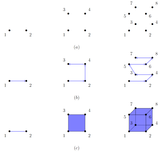
The figure above shows how connectivity is defined for a region in each dimension. Fig (a) shows the gridpoint structure for these regions and Fig (c) shows how the resulting mesh appears. Fig (b) shows how a connectivity list should be sequenced to create the desired mesh. Then, in 1D, our connectivity list to create the line in (c) would be [1,2]. Similarly, in 2D, our connectivity list would be [1,2,4,3] and in 3D, our list would be [1,2,4,3,5,6,8,7]. (Note that this sequencing is dictated by Paraview's conventions, not SpECTRE's.)
The above example illustrates how to connect the smallest connected region in each dimension. The complete connectivity list, detailing how the entire domain mesh is to be created, is made by concatenating individual connectivity lists. Thus, in 1D, Paraview interprets the list [1,2,2,3] in blocks of 2, with the first block [1,2] representing a line between gridpoints 1 and 2, and the second block [2,3] representing a line between gridpoints 2 and 3. This works similarly in the other dimensions.
How does ExtendConnectivity work?
ExtendConnectivity is a post-processing algorithm that looks to add more connectivity entries to fill up any gaps in visualisation. These gaps have multiple sources, the largest of which is the fact that SpECTRE does not add connectivity between elements (as defined in Domain Concepts) by default. This is important in certain simulations where the endpoints of the elements do not overlap (e.g simulations using Gauss quadrature), resulting in gaps between elements in visualisations. ExtendConnectivity looks to fix this problem specifically. Note: The remainder of this guide assumes we are working with simulations whose elements don't overlap.
Neighbours
The key idea in understanding how ExtendConnectivity works is understanding how neighbouring elements are categorised and dealt with. The next sections explain the categories of 'face neighbour', 'edge neighbour', and 'corner neighbour' in detail for 1D, 2D, and 3D.
3D
We shall start in 3D because the categories are most intuitively defined in 3D. The image below shows a typical example of SpECTRE connectivity for a 3D volume element (with h-refinement 1 and p-refinement 2 in each direction), coloured by their neighbour categorisation.
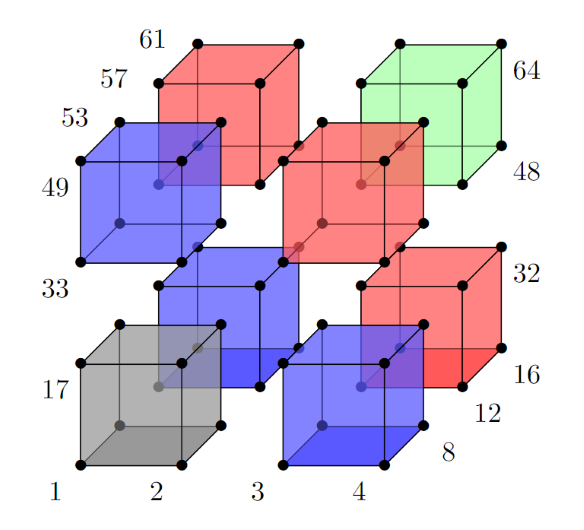
In the above image, the grey cube is our reference element that neighbour elements are defined around. Then, we define any element that, if elements overlapped, would share a face with our reference element to be a 'face neighbour'. By this definition, we can see that our blue cubes in the above image are our face neighbours. The definitions of the other categories are analogous. We define any element that, if elements overlapped, would share an edge to be an 'edge neighbour' and any element that would share a corner to be a 'corner neighbour'. Hence, our red cubes are our edge neighbours and our green cube is our corner neighbour. In general, for a 3D simulation, face neighbours share a 2D region, edge neighbours share a 1D region, and corner neighbours share a 0D region.
These categories apply to the element as a whole. Then, after the element is categorised, the gridpoints must be filtered to the particular face, edge, or corner that will be connected with our reference element. Note that edge and corner neighbours require gridpoints from multiple neighbours (e.g. edge neighbours involve connecting four edges - one from the reference element, two from face neighbours, and one from the edge neighbour). Once the correct gridpoints are identified, they are connected as described in the previous section. The neighbour direction in particular determines the ordering of the gridpoints in this sequence. The image below shows the same domain after the missing connectivity has been added, coloured by the type of connectivity added.
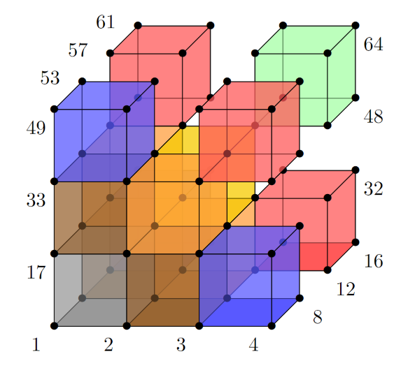
In this image, the brown cubes are the face neighbour connections, the orange cubes are the edge neighbour connections, and the yellow cube is the corner neighbour connection. The entire process is then repeated for the next element.
This example required only one connectivity entry to be added per neighbour since each element was made up of just one cube. At larger p-refinements, an element consists of more cubes and consequently, more connectivity entries are required. For example, if the domain above had a p-refinement of 3 in each dimension instead, face connections would require adding four cubes and edge connections would require two cubes.
2D
We can now generalise these definitions to other dimensions. The image below shows a typical example of SpECTRE connectivity for a 2D volume element (with h-refinement 1 and p-refinement 2 in each direction), coloured by their neighbour categorisation in the same colours as above.
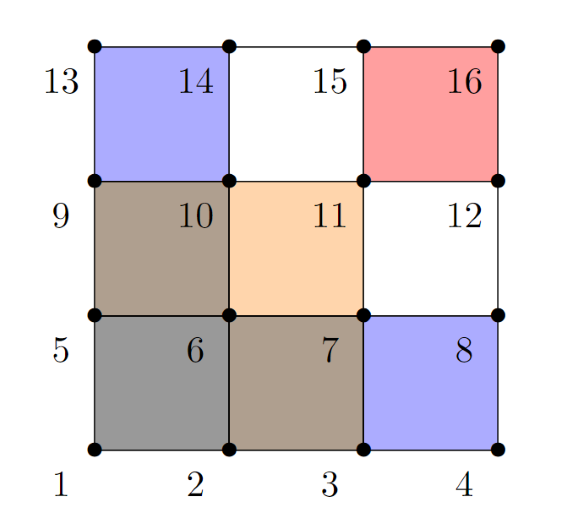
Once again, the grey square is our reference element. We now define our neighbour types to be analogous to the types in 3D but reduced by one dimension. Then, in a 2D simulation, face neighbours share a 1D regions, edge neighbours share a 0D region, and corner neighbours do not exist. In the image above, our face neighbours are once again blue and our edge neighbours are once again red.
Once the elements are categorised, the relevant gridpoints are once again filtered and connected according to the 2D structure explained above. In the image, the face connections are coloured brown and the edge connections are coloured orange again. The next element is then made the reference element and the process is repeated to build up the connectivity for the entire domain.
1D
We display the concepts in 1D for completeness. The image below shows an example of SpECTRE connectivity for a 1D volume element (with h-refinement 1 and p-refinement 2), coloured by their neighbour categorisation in the same colours as above.
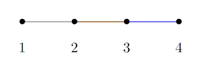
In this image, the grey line is our reference element. In a 1D simulation, we correspondingly define face neighbours to share a 0D region and both edge and corner neighbours do not exist. Then, in the image above, our face neighbour is once again the blue element and the face connection is coloured brown again.
Summary
- Face Neighbour:
A neighbouring element that shares an overlap region one dimension lower than the dimension of the simulation. - Edge Neighbour:
A neighbouring element that shares an overlap region two dimensions lower than the dimension of the simulation. - Corner Neighbour:
A neighbouring element that shares an overlap region three dimensions lower than the dimension of the simulation.
Connecting elements with different p-refinements
To be added.