Introduction
The simplest way to construct a volume map from two parameterized surfaces is by linearly interpolating between them:
\[\vec{x}(\xi,\eta,\zeta) = \frac{1-\zeta}{2}\vec{\sigma}_-(\xi,\eta)+ \frac{1+\zeta}{2}\vec{\sigma}_+(\xi,\eta)\]
In the above example, each surface \(\vec{\sigma}_+\) and \(\vec{\sigma}_-\) is parameterized using the logical coordinates \(\xi\) and \(\eta\), and a third coordinate \(\zeta\in[-1,1]\) is used to interpolate between them.
We then distribute gridpoints on this volume by specifying values of the coordinates \(\xi,\eta,\) and \(\zeta\) at which the gridpoints are located. In SpECTRE these values are the locations of the quadrature nodes. The distribution of the gridpoints throughout the volume depends on the parameterization used, and the simplest choice of parameterization does not necessarily lead to the best gridpoint distribution. In this section we discuss situations in which there exist better parameterizations than those obtained by linear interpolation.
Generalized Logical Coordinates
In each of the following examples, we will obtain functions \(\Xi(\xi), \mathrm{H}(\eta),\) and \(\mathrm{Z}(\zeta)\) that give better gridpoint distributions than using the logical coordinates alone. Where possible, we will write the reparameterized map such that the functional form of the map is unchanged when replacing \(\Xi\) with \(\xi\), etc. We therefore refer to \(\Xi, \mathrm{H},\) and \(\mathrm{Z}\) as the generalized logical coordinates, as they can also refer to the logical coordinates \(\xi, \eta,\) and \(\zeta\) themselves, when the transformation is the identity.
Equiangular Maps
The mapping for a cubed sphere surface can be easily obtained by taking points that lie on each face of a cube and normalizing them such that they lie on the sphere:
\[\vec{\sigma}_{+z}(\xi,\eta) = \frac{1}{\sqrt{1 + \xi^2 + \eta^2}} \begin{bmatrix} \xi\\ \eta\\ 1\\ \end{bmatrix}\]
In the above example the parameterization used for the upper \(+z\) surface of the cube is linear in \(\xi\) and \(\eta\). However, distances measured on the surface of the sphere are not linear in \(\xi\) and \(\eta\). To see this, one may compute \(g_{\xi\xi} = |\frac{\partial\vec{x}}{\partial\xi}|^2\) to see how distances are measured in terms of \(\xi\):
\[g_{\xi,\xi}|_{\eta=0} = \frac{1}{(1+\xi^2)^2}\]
This metric term demonstrates that a gridpoint distribution uniform in \(\xi\) will end up being compressed near \(\xi=\pm1\). Suppose we reparameterized the surface using the generalized logical coordinate \(\Xi\in[-1,1]\). We would find:
\[g_{\xi,\xi}|_{\eta=0} = \frac{\Xi'^2}{(1+\Xi^2)^2}\]
Ideally, we would like distances measured along a curvilinear surface to be linear in the logical coordinates. We solve the differential equation and obtain:
\[\Xi = \tan(\xi\pi/4)\]
These two parameterizations of the cubed sphere are known as the equidistant and equiangular central projections of the cube onto the sphere. We now summarize their usage in SpECTRE CoordinateMaps that have with_equiangular_map as a specifiable parameter:
In the case where with_equiangular_map is true, we have the equiangular coordinates
\[\textrm{equiangular xi} : \Xi(\xi) = \textrm{tan}(\xi\pi/4)\]
\[\textrm{equiangular eta} : \mathrm{H}(\eta) = \textrm{tan}(\eta\pi/4)\]
with derivatives
\[\Xi'(\xi) = \frac{\pi}{4}(1+\Xi^2)\]
,
\[\mathrm{H}'(\eta) = \frac{\pi}{4}(1+\mathrm{H}^2)\]
In the case where with_equiangular_map is false, we have the equidistant coordinates
\[ \textrm{equidistant xi} : \Xi = \xi\]
\[ \textrm{equidistant eta} : \mathrm{H} = \eta\]
with derivatives:
\[\Xi'(\xi) = 1\]
\[\mathrm{H}'(\eta) = 1\]
Projective Maps
The mapping for any convex quadrilateral can be obtained by bilinearly interpolating between each vertex \(\vec{x}_1, \vec{x}_2, \vec{x}_3\) and \(\vec{x}_4\):
\[\vec{x}(\xi,\eta) = \frac{(1-\xi)(1-\eta)}{4}\vec{x}_1+ \frac{(1+\xi)(1-\eta)}{4}\vec{x}_2+ \frac{(1-\xi)(1+\eta)}{4}\vec{x}_3+ \frac{(1+\xi)(1+\eta)}{4}\vec{x}_4 \]
In the case of a trapezoid where two of the sides are parallel, it is appropriate to linearly interpolate along the parallel sides. However, linearly interpolating between the two bases results in a less than ideal gridpoint distribution. This happens in the case of SpECTRE's Frustum, where the logical coordinate \(\zeta\) interpolates between the bases.
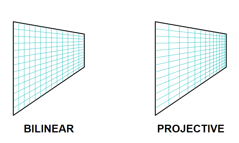
As seen in Veltman's [Warp-Off] (https://bl.ocks.org/veltman/8f5a157276b1dc18ce2fba1bc06dfb48), linear interpolation between the two bases results in a uniformly spaced grid between the bases of the frustum. This causes elements near the smaller base to be longer in the direction normal to the base, and elements near the larger base to be shorter in the direction normal to the base. We desire elements that have roughly equal sizes along each of their dimensions.
We can redistribute the gridpoints in the \(\zeta\) direction using a projective map, moving more gridpoints toward the smaller base. We can also see in the figure above that a projective map can be applied incorrectly, leaving elements distorted at the opposite end. From this we can see that it is important to control the degree of projection.
We adapt a technique from projective geometry to obtain the desired grid spacing. The heart of the method lies in the fact that objects arranged in a line at equal distances from one another will appear to converge as they approach the horizon.
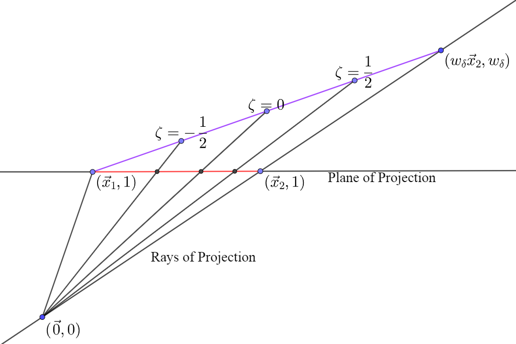
The above diagram demonstrates how to obtain a nonlinearly parameterized object (seen in red) from a linearly parameterized one (seen in purple). This is done by lifting the linearly parameterized object into a higher spatial dimension \(w\), such that its projection onto the plane remains unchanged. As seen above, \(w_{\delta}\) controls the degree of projection of one end of the object (purple) into a higher spatial dimension \(w\). In projective geometry, these points that exist in the higher dimension are labeled with homogeneous coordinates \(\tilde{x}, \tilde{y}, \tilde{z}, w\), to distinguish them from the Cartesian coordinates that label points that exist on the \(w=1\) hyperplane, \(x,y,z\). The resulting grid (seen in red) is obtained by projecting back into the \(w=1\) hyperplane. The Cartesian coordinates are obtained by dividing each homogeneous coordinate of the linearly parameterized object by its respective \(w\) coordinate value.
The parametric equation for the purple object seen above in homogeneous coordinates is:
\[\begin{bmatrix}\tilde{x}\\\tilde{y}\\\tilde{z}\\w\\\end{bmatrix}= \frac{1-\zeta}{2}\begin{bmatrix}x_1\\y_1\\z_1\\1\\\end{bmatrix}+ \frac{1+\zeta}{2}\begin{bmatrix}x_2w_{\delta}\\y_2w_{\delta}\\ z_2w_{\delta}\\w_{\delta}\\\end{bmatrix}\]
The equation for the projected red object in Cartesian coordinates is obtained by dividing by w:
\[\vec{x}(\zeta) = \frac{1}{w(\zeta)} \begin{bmatrix} \tilde{x}(\zeta)\\ \tilde{y}(\zeta)\\ \tilde{z}(\zeta)\\ \end{bmatrix}\]
We wish to cast our parametric equation for the surface into the form:
\[\vec{x}(\zeta) = \frac{1-\mathrm{Z}}{2}\vec{x}_1 + \frac{1+\mathrm{Z}}{2}\vec{x}_2\]
for some appropriate choice of auxiliary variable projective_zeta \( = \mathrm{Z}(\zeta)\). We would also like for \(\mathrm{Z}\) to reduce to \(\zeta\) when \(w_{\delta}\ = 1\).
Defining the auxiliary variables \(w_{\pm} := w_{\delta}\pm 1\), the desired \(\mathrm{Z}(\zeta)\) is given by:
\[\mathrm{Z} = \frac{w_- + \zeta w_+} {w_+ + \zeta w_-}\]
with derivative:
\[\mathrm{Z}' = \frac{\partial\mathrm{Z}}{\partial \zeta} = \frac{w_+^2 - w_-^2}{(w_+ + \zeta w_-)^2}\]
For SpECTRE CoordinateMaps that have projective_scale_factor as a specifiable parameter, the value \(w_{\delta} = 1\) should be supplied in case the user does not want to use projective scaling. If auto_projective_scale_factor is set to true, the map will compute a value of \(w_{\delta}\) that is appropriate.