SpECTRE can be a bit complicated to get started with, especially if you aren't familiar with our core concepts of task-based parallelism and Template Meta-Programming (TMP). However, Don't Panic. This guide aims to get you introduced to running, visualizing, editing, and then rebuilding SpECTRE to give you a feel for what SpECTRE is all about, all on your own laptop! Hopefully by the end of this guide you'll feel comfortable enough to look at other executables and maybe even venture into the code itself!
Prerequisites
To start off, you'll need to obtain an environment to build and run SpECTRE in. You could try and install all the dependencies yourself, but that is very tedious and very error prone. Instead, we provide a Docker container with all the dependencies pre-installed for you to use. The container also has the SpECTRE repository cloned in it already so you don't have to worry about getting it yourself. To obtain the docker image, run
Another program you will need for this tutorial is Paraview for visualizing the output. You specifically will need version 5.10.1 for this tutorial.
If you'd like to use VSCode, the tutorial also has instructions for how to start in VSCode as well.
Into the Container
For both a terminal and VSCode, create the container in a terminal and start it.
We connect port 11111 on your local machine to port 11111 of the container so we can use Paraview. The --rm will delete the container when you stop it. This won't put you into the container, only start it in the background.
- Note
- The --entrypoint "/bin/bash" is important because the default entrypoint of the container is the SpECTRE CLI. You can try out the default entrypoint by running docker run sxscollaboration/spectre:demo -h and it'll print the help string for the CLI. See the Python documentation for more.
You can also run a Jupyter server for accessing the Python bindings (see Using SpECTRE's Python modules) or running Jupyter notebooks. To do so, append another -p option with your specified port, e.g. -p 8000:8000. You can chain as many -p options as you want to expose more ports.
The SpECTRE repository is located at /work/spectre inside the container.
With a Terminal
To hop in the container from a terminal, simply type
and now you're in the container!
With VSCode
If you're using VSCode, you'll need the Remote-Containers extension to be able to access the container. Once you have it, open the command palette and run the following commands.
- Remote-Containers: Attach to Running Container - you should see the container spectre_demo that's currently running. Select that.
- File: Open Folder - select /work/spectre which is where the repo is.
Now you're in the container within VSCode! The terminal in VSCode will look identical to the one if you hadn't used VSCode.
- Note
- Any changes you make inside /work/spectre will be lost once you stop the container. If you'd like your changes to persist, get rid of the --rm flag in the docker create command.
Compiling the code
- Note
- From here on out, all paths are assumed to be inside the container unless specified otherwise.
The container already has a SpECTRE build pre-configured. Go to the build directory and compile the executables that we will use in this tutorial:
This will compile the code on two cores. If you'd like to use more cores, use the -j N option where N is the number of cores.
Once the executables are compiled they will be available in the /work/spectre/build/bin directory. The container already has this directory added to the PATH environment variable, so you can run executables from the command line right away:
If you are not in the container but instead on a desktop or cluster you can add the bin directory to your path by cding to the build directory and running
If you log out and log back in you will need to set this again, unless you add it to your shell's init file.
Running ExportCoordinates3D
First we will run the ExportCoordinates3D executable to visualize the coordinates of a binary black hole domain. Make a directory where you will run everything:
Copy over the input file /work/spectre/tests/InputFiles/ExportCoordinates/InputTimeDependent3D.yaml into your /work/runs directory. To run the executable, do
This will run it on 4 cores (the --no-schedule means it will run on the login/head node if you are using an HPC system). After this finishes you should see two H5 files in your run directory:
- ExportCoordinates3DVolume0
- ExportCoordinates3DReductions
The Volume file is where we store data from every element in our domain, like the coordinates or the metric. The Reductions file is for more global quantities like the minimum grid spacing over all the elements in our domain.
- Note
- Next time you run the executable, you will have to either move or delete the existing H5 files as SpECTRE will error if it detects that an output file already exists. This is to prevent you from accidentally overwriting data. You can also use the --force / -f and --clean-output / -C flags to have spectre run delete the existing files before running the executable.
Visualizing our BBH Coordinates
Now it's time to use Paraview to visualize the coordinates we use for our BBH evolutions! SpECTRE will actually export the physical frame coordinates for every executable we have because they are a really useful diagnostic to have. We are just using the ExportCoordinates executable here so that you don't have to run a BBH evolution on your laptop which probably wouldn't work because of memory requirements.
Before we get to Paraview, we have to tell paraview how to actually use the coordinates in the Volume H5 file. To do this we have a tool called generate-xdmf in our Python command-line interface. Inside the runs directory where you have the H5 files, run
We output volume data per node so we append the node number to each volume file we have. Since you're most likely running on a laptop, you'll only be running on one node so you should only get one output file for the volume. The --subfile-name argument is the group name inside the H5 file where the data is stored (groups can be checked by h5ls -r FILE_NAME). generate-xdmf will generate a file called BBH_Coords.xmf. Make sure to keep this .xmf file next to the volume file it was generated from. It uses relative paths to find the volume file which means if you move it, you won't be able to visualize anything.
Attaching Paraview
This is where we actually need Paraview. We have a headless (no GUI) vesion of paraview inside the container which we will refer to as the "server". To start the Paraview server, run
- Note
- For cluster users, check cluster-specific instructions for ParaView. You may require MPI and specify which port to use. You can run mpirun -np 1 pvserver -p PARAVIEW_REMOTE_PORT on the remote cluster. Here, PARAVIEW_REMOTE_PORT is the port that the ParaView server will use on the cluster. You may choose it to be, for example, 11112. With 'pvserver' running on the remote machine, open a new local terminal. Locally, run ssh -L11111:YOUR_CLUSTER:PARAVIEW_REMOTE_PORT USERNAME@YOUR_CLUSTER.
The & is so that the server runs in the background. If you hit Enter a couple times you'll get back to being able to type commands. You should see some output similar to
This means it's waiting for you to connect some external Paraview session (the "client") to the server. Now, outside the container, start a session of Paraview 5.10.1. (Again, you must use this version otherwise it won't work properly.)
- Note
- For cluster users, run mpirun -n 1 pvserver --version to check ParaView version. On your computer, download exactly the same version of Paraview.
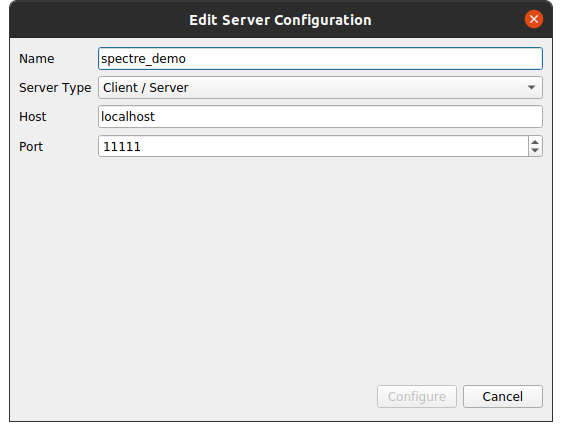
Go to File > Connect. Click Add Server. Name it whatever you want, but keep the Host as localhost, the Server Type as Client/Server, the Port as 11111 (remember the -p 11111:11111 flag from the docker command?). Here's a snapshot of what it should look like before you configure.
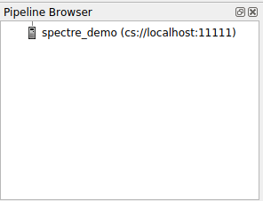
Hit Configure, then hit Save (we don't care about the launch configuration). Now you should see a list of your configured servers. Select the one you just created and hit Connect. It may take a minute or two to connect to the server, but once you do on the left you'll see something like
- Note
- If you close your client, the server will stop and you won't be able to reconnect. You'll have to restart the server in the container.
Open the XMF File in Paraview Client
Now that you have Paraview connected to the container, open the BBH_Coords.xmf file you just generated inside Paraview (the paths you'll see are the ones in the container, not your filesystem). You may be prompted to choose which XDMF reader to use. Choose the XDMF Reader option. The Xdmf3 options won't work. Once you choose a reader, on the left, you'll see
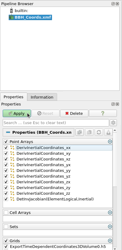
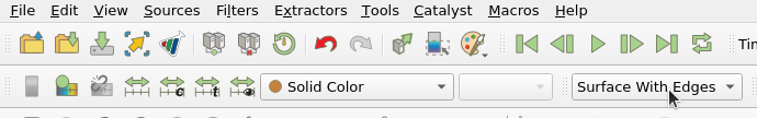
You can uncheck all the boxes in the Point Arrays section as they aren't necessary for visualizing the coordinates. Then hit Apply. Now you should see a solid sphere. This isn't super helpful. In the top bar you should see a dropdown to change the style that the points are plotted in. Select Surface With Edges like so. (Note: Your top bar may look slightly different from this depending on what version of Paraview you have.)
Now you'll have a solid sphere with highlighted lines. To view the interior of the domain, you'll need to add a filter. To access the filters, navigate to Filters on the top menu bar, hover over Alphabetical, and search for your filter of choice. Probably the two most helpful filters for viewing the domain are the Slice and Clip filters. (Note that you'll have to choose the Surface With Edges option for each filter separately.)
Slice is fairly self explanatory in that it will show you a single plane through the domain. Experiment with different planes to see our whole domain structure!
The Clip filter will remove all points "above" a certain plane, where "above" is in the direction of the normal of that plane. If you combine two orthogonal Clips, you can actually view a 3D wedge of our domain. Try moving the centers of the planes to view the domain around our excision surfaces! They have a lot of cool structure.
If you'd like to read more about our BBH domain, you can look at the documentation for domain::creators::BinaryCompactObject.
Evolution of BBH Coordinates
Now that you are able to export and visualize our BBH domain coordinates at a single time, let's make a small movie of the coordinates as they evolve! To do this, we'll need to edit the input file InputTimeDependent3D.yaml. If you aren't familiar with YAML, it's a file type that uses key-value pairs to create actual objects in our C++ code. Feel free to experiment with keys and values in our input files. If you're unsure about what a key or value should be, we offer an easy way to check the options in the input file without running a whole simulation. In your /work/runs directory, if you run
the executable will parse and check the input file. If you made a typo, or added an incorrect key/value, a list of the available keys and their associated values will be printed.
To change the number of times we output the coordinates, we'll need to go to the EventsAndTriggers: block of the input file. This block is mainly where we specify which quantities we want to observe in a simulation or where we "Trigger" a specific "Event" to happen. (For more info on EventsAndTriggers, see the Events and triggers tutorial.) Currently in this input file we only have one Trigger/Event pair. The Trigger is TimeCompares: and the Event is Completion. To have the simulation run longer, change the Value: under TimeCompares: to something larger. If you look at the Evolution: block above the EventsAndTriggers: block, you'll see that the initial time step is 0.5. The way this executable is set up, the coordinates will be exported every time step. So set the final time Value: under TimeCompares: to some larger multiple of 0.5 so that you'll have the coordinates at a bunch of different times (a final time of 20 is reasonable. Depending on how many cores you run on this should take a couple minutes).
Then, run the executable just like you did above (remember to move or delete the existing H5 files), run generate-xdmf, and open it in Paraview and apply some filters of your choice. We recommend using a Slice filter with the normal pointing in the -z direction. This is because our BBH domain rotates about the z axis. Now, in the top bar of Paraview, you should see a "Play" button that looks like a sideways triangle (see the second image in the Open the XMF File in Paraview Client section). If you click this, Paraview will step through all the timesteps in the output files and you'll be able to see the domain rotate a bit!
Next, we encourage you to play with the other inputs that control how the domain evolves over time. These options are housed in the
block of the input file. Since this tutorial is more about running the code, we won't go into too much detail about each option. However, in general:
- ExpansionMap is a global map (all parts of the domain) that controls the separation between the excision surfaces
- RotationMap is a global map that controls how the excision spheres rotate about each other
- SizeMap is a local map only around the excision spheres (not in the wave zone) that control the compression of grid points.
Play around with these values! You may get an error if you put something that's too unphysical, but this is a fairly consequence-free playground for you to explore so just try a different value.
Now you have a movie of how BBH coordinates evolve in a SpECTRE simulation!
Exploring DG+FD
Now that you are able to run, and visualize SpECTRE, let's explore a feature that is fairly unique to SpECTRE and is really powerful for handling discontinuities and shocks in our simulations. We call this feature DG+FD (it's also sometimes referred to as just subcell).
Description of DG+FD
FD is the usual finite difference you are used to. All of the BSSN codes use finite difference for solving Einstein's equations. FD is very good at capturing shocks and discontinuities and is a very robust method, making it well suited for hydro problems and other systems that have shocks and discontinuities.
DG stands for Discontinuous Galerkin. DG is a spectral method for representing a solution on a grid, meaning that instead of taking the difference between the function value at two points to get the derivative, it uses known basis functions to represent the solution. Then the derivative can be known analytically and you only need to supply the coefficients for the basis. DG works best for representing smooth solutions; ones with very few shocks and discontinuities (like GR in vacuum). This makes DG much faster than FD for smooth solutions.
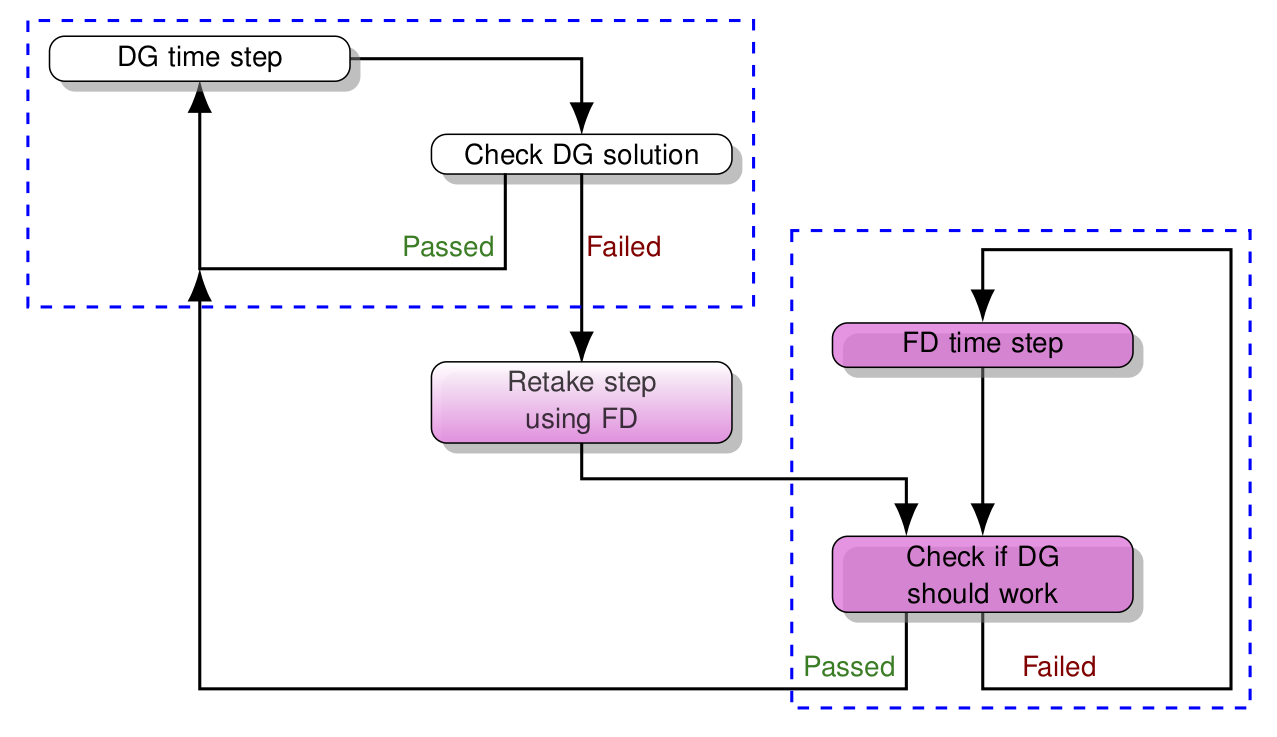
In SpECTRE, we combine these two different methods into one system to take advantage of the strengths of each. When we have a solution that is smooth in some parts of the domain, but has shocks in other parts, using only one of these methods has disadvantages. If we only used DG, we wouldn't be able to resolve the shocks very well driving the errors up a lot. If we only used FD, we'd be able to represent the solution well, but it would be computationally inefficient. So we combine DG+FD so that we only do DG in the parts of the domain where the solution is smooth, and switch to FD in parts where there may be a shock or discontinuity. The algorithm for switching between DG and FD is explained in this image.
If you'd like to learn more about how SpECTRE implements its DG+FD scheme, you can read the paper on the ArXiv.
Running the Kuzmin Problem
To demonstrate DG+FD, we will be evolving the Kuzmin problem using the EvolveScalarAdvection2D executable. This is a simple test problem that rotates a set of geometric shapes with uniform angular velocity, which can be used to evaluate how well a numerical code can handle discontinuities stably over time. Inside the container make a new directory /work/runs2 where you will run it. Also copy the default input file in /work/spectre/tests/InputFiles/ScalarAdvection/Kuzmin2D.yaml to this new /work/runs2 directory.
Changing the Default Input File
The default input file has very low resolution so we'll need to crank that up a bit. The way to do this is to change the initial refinement levels and initial number of grid points which are located in
InitialRefinement: represents how many times we split a Block in half in order to create Elements, which are the fundamental units of our domain. So an initial refinement of [1, 1] means we split a single Block into 4 elements (split in half once in each direction). For an initial refinement of [2, 2] we first do 1 refinement like before, and then split each of the resulting 4 elements in half again in each direction, resulting in 16 total Elements. To determine the total number of Elements for a given refinement (same in all directions), just do \(2^{\mathrm{Dim * Refinement}}\). If you're confused by the terminology we use to describe the domain, we have a Domain Concepts guide that explains all terms related to our domain.
InitialGridPoints represents the number of grid points per dimension in each Element after the final refinement has been applied. So if we had an initial refinement of [2, 2] like above and then initial grid points [3, 3] in each Element, we'd have a total of 9x16=144 grid points.
As for actual numbers to use, you can experiment to see what gives good, well-resolved results. You'll definitely need more refinement than the default input file, but since refinement scales exponentially, this can become very expensive very quickly. On a laptop, you probably shouldn't go higher than refinement [6, 6]. As for grid points, this will depend on how much refinement you have. If you have a ton of small elements, you won't need too many grid points to resolve the solution; something like [4, 4] would work. If you don't have a lot of refinement, you may want more grid points if you still want to resolve your solution. For a DG scheme, increasing the number of grid points (p refinement) reduces the numerical error exponentially where the solution is smooth, so computational resources are used more effectively. However, to resolve shocks and discontinuities we have to refine the domain into more and smaller elements instead (h refinement). Striking the most effective balance between h and p refinement in different parts of the domain is the job of an adaptive mesh refinement (AMR) algorithm.
The default input file only runs for a few time steps so we'll want to make this run longer so we can actually see some evolution. From the documentation of the Kuzmin system, the solution will rotate with an angular velocity of 1.0 (in code units). Thus, to do a full orbit, it will take 6.28 code units of time. In the EventsAndTriggers: block of the input file, we see that the Completion event is triggered by the Slabs trigger. We could, in theory, calculate out how many slabs 6.28 code units is using the time step, but that's super tedious. Instead let's trigger completion using the TimeCompares trigger instead. We used this before when exporting the BBH coordinates, so just copy over the yaml block and change the Value:.
Your final EventsAndTriggers: block should look something like this:
Now you should be ready to run the executable and get some output. Here, you will almost definitely benefit by running this on many cores by adding the -j N flag to the command you use to run the executable. Since we use lots of smaller elements, we distribute these over the available resources via a space filling curve to speed things up.
Visualizing the Kuzmin Problem
Once your run finishes, extract the volume data with generate-xdmf using
(Note that the subfile-name is different than before because it was different in the input file) and load it into Paraview once again. We are only interested in the quantity U which is the scalar field we were evolving. You can uncheck any other boxes. So now, instead of coordinates on your screen, you should see a large square colored by the solution profile described in the Kuzmin system. You should also notice that there are smaller squares that don't touch each other in the middle of the domain and on the edges there are large sections that are continuous. These are the FD and DG grids, respectively. If you go to the top bar in Paraview and change how you view the grid to Surface With Edges, this will become even more apparent.
You will notice that the FD grid is mostly around where the interesting features are in the solution profile; the cylinder with a wedge cut out, the cone, and the hump. And then the DG grid is mostly where the solution should be zero towards the boundary of the domain (i.e. the very smooth part). So right from the start, you can see that we are saving computational effort by only doing the expensive, yet robust, method (FD) where it is necessary and the efficient method (DG) everywhere else where the solution is smooth.
Now hit the "Play" button in the top bar of Paraview and watch the solution evolve. You'll notice that the elements in the domain switch back and forth between FD and DG. They do so in such a way that the elements will switch to FD when an interesting feature enters the element and then switch back to DG once the feature leaves. In this way, we are able to actually track shocks and discontinuities in real time in our solution by where the code switches to using FD instead of DG. This is extremely useful for expensive GRMHD simulations where we only want to do FD at a shock boundary, yet that shock boundary is moving through the domain. We are able to dynamically track this shock and resolve it well with FD, then switch back to DG after the shock passes through and the solution has settled down again.
A pretty cool filter you can add is Warp By Scalar. In the left panel, choose the solution variable U as the scalar to use and hit Apply. In the viewing panel there should be a 2D or 3D button that you can toggle to make the view 3D. Once you do that you should be able to see that the height of the feature is your solution U. If you change the grid to Surface With Edges you can see the FD or DG grids warp with the solution. And if you hit "Play" it'll rotate around and you'll see the features moving in 3D! (Don't worry if you can't find this filter. Not all versions of Paraview may have it.)
We encourage you to play around with the refinement and grid points before the next section to get a feel for how each changes the runtime and accuracy of solution.
Editing the Kuzmin System
Hopefully now you feel comfortable enough running SpECTRE that you can get the default input file for the pre-built executables, edit it, and run it. Now we are going to try our hand at actually editing some code in SpECTRE and then building SpECTRE. We're going to stick with the Kuzmin system and add a new feature to the solution profile!
You can find the files for the Kuzmin system at /work/spectre/src/PointwiseFunctions/AnalyticSolutions/ScalarAdvection/ Kuzmin.?pp. In the hpp file, you'll see a lot of Doxygen documentation and then the actual Kuzmin class. The only function that you will need to care about is
All of our analytic solutions have a function similar to this that will set the value corresponding to the tag in the return type. If you're unfamiliar with tags in SpECTRE, you can look at these sections for an explanation, A TaggedTuple DataBox and SpECTRE's DataBox. However, it's basically just a fancy way of doing a compile-time key/value pair. The tag is the key, and the value is whatever you want it to be. In our case, the value is a tensor, representing the solution.
The definition of this function in the cpp file is where you will be editing the actual Kuzmin solution. Towards the bottom of this function, there is a for loop that sets the solution at every grid point. This is where you will add in a new feature to the solution.
You can pick any feature you want to add, so long as it's inside the domain bounds of [0,1]x[0,1] and centered around (0.75, 0.5). This is because of how the kuzmin solution is set up with existing features at (0.25, 0.5); (0.5, 0.25); (0.5, 0.75). If you're having trouble thinking of a feature to add try one of the following features:
- Square centered at (0.75, 0.5) with solution value 1.0
- Side length 0.1 (any larger and it might interfere with the other features)
- Circle of radius 0.045 centered on the square with value 0.0
- Triangle centered at (0.75, 0.5) with one corner facing in the +x direction with solution value 1.0
- Square centered at (0.75, 0.5)
- Side length 0.1 (any larger and it might interfere with the other features)
- Left half of the square has value 1.0 and right half of the square has value 0.5
- Note
- The more detailed you make your feature, the more resolution you will need to resolve it.
Re-building SpECTRE
Once you have your feature coded up, go ahead and save your changes. Now we will build SpECTRE! Go to the /work/spectre/build directory. This is where you have to be in order to build SpECTRE. We use CMake to configure our build directory. However, since the executables are already pre-built, this means the build directory is already configured! So you don't have to worry about CMake for now. If you wanted to reconfigure, for example using a different compiler, then you'd have to run CMake. If you want to learn more about how we use CMake, take a look at the Commonly Used CMake flags developers guide.
To build the Kuzmin executable, run
This should be very fast because you only edited a cpp file. Congrats! You've just built SpECTRE!
Now re-run the executable in your /work/runs2 directory. Hopefully everything works and you get some output. When you plot it in Paraview, it should look almost the same as before except your feature will be there too rotating with the others! How cool! You can also see if your feature needs FD or DG more by how much it switches back and forth.
Experiment some more with either different features or different resolution!
Conclusions
Congrats! You've made it through the tutorial! If you only want to run our pre-built executables, you have all the tools necessary to run, visualize, and re-build them. If you want a full list of our executables, do make list in the build directory. This will also include our Test_ executables which you can just ignore.
In an already configured build directory, all you have to do to build a new executable is
and then you can copy the default input file from /work/spectre/tests/InputFiles and run it. Running an executable with the --help flag will give a description of what system is being evolved and the input options necessary.